
Lookup Based on Multiple Criteria
The following examples illustrate how to perform a lookup based on multiple criteria. The first example uses an array formula, thereby avoiding the use of a helper column. However, the second example uses a helper column and avoids the need for an array formula.
Without Using a Helper Column
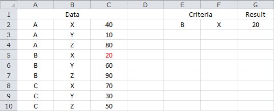
The following formulas return a value from C2:C10, where the corresponding value in A2:A10 equals the value in E2, and the corresponding value in B2:B10 equals the value in F2...
=INDEX(C2:C10,MATCH(1,IF(A2:A10=E2,IF(B2:B10=F2,1)),0))
or
=INDEX(C2:C10,MATCH(E2&"#"&F2,A2:A10&"#"&B2:B10,0))
Note that these formulas need to be confirmed with CONTROL+SHIFT+ENTER. If done correctly, Excel will automatically place curly braces {...} around the formula.
Based on the sample data, the formula returns 20.
Sample Workbook: Download
Using a Helper Column
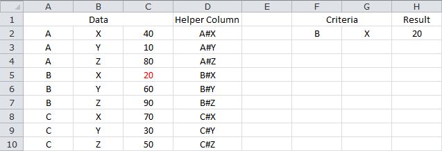
First, the following formula is entered in D2 and copied down so that each value in A2:A10 is concatenated with its corresponding value in B2:B10...
=A2&"#"&B2
Then, the following formula returns a value from C2:C10, where the corresponding value in D2:D10 equals the concatenated value of F2 and G2...
=INDEX(C2:C10,MATCH(F2&"#"&G2,D2:D10,0))
Sample Workbook: Download